Mathematical Derivation and Python Implementation of Principal Component Analysis

Dimensionality reduction is the transformation of data from a higher dimensional space to low-dimensional space, such that the information loss is minimum. Dimensionality reduction can be used for noise reduction, data visualization, cluster analysis, or as an intermediate step to facilitate other analyses. Principal Component analysis(PCA) is one such technique.

In PCA, we reduce n-dimensional data to a lower q-dimensional representation, by projecting the data along q orthonormal vectors(principal components) such that the average squared Euclidean distance (L2 norm) between the original data points and the projected points is minimum.

Equivalently, we will find that it is the same as trying to find a subspace of q-dimensions such that the variance of projected data along the vectors of the orthonormal basis consisting of the principal components is maximized.

While deriving, we will come across the assumption of the data being centred. It’s a crucial assumption and if not, then the data should be centered first by subtracting the mean.

In the end, we will conclude by proving that the principal components are the eigenvectors of the sample covariance matrix, and the eigenvalues are the variance in the directions corresponding to the principal components.

Linear algebraic preliminaries

Let $V$ be any finite vector space, with inner product $\langle.,.\rangle$.

Definition: For any subset of vectors, $S \subseteq V$, the orthogonal subspace of S, $S^\perp$ is defined as,

Theorem 1: For any subspace $W$ of $V$, $V$ is the direct sum of $W$ and $W^\perp$.

Proof: Let $x \in W \cap W^\perp$. Then, by definition of orthogonal subspace, $\langle x,x \rangle=0$. It implies that $x$ is the zero vector. Therefore, $W \cap W^\perp = \lbrace 0_v \rbrace$. (Result 1)

Let $x \in V$, $\beta$ be an orthonormal basis of $W$.

Therefore, $\beta = \lbrace v_1,v_2,v_3…v_m \rbrace$ such that $\langle v_i,v_i \rangle = 1$ and for $i \neq j$, $\langle v_i,v_j \rangle = 0$.

Let $w \in W$ such that,

$\Rightarrow$ for any $v_i \in \beta$, $\langle x-w, v_i \rangle=0$

$\Rightarrow$ $x-w \in W^\perp$

$\Rightarrow$ $x=w+(x-w) \in W \cup W^\perp$

Therefore, $V=W \cup W^\perp$ (Result 2)

Combining the results (Result 1) and (Result 2), we prove the theorem.

Note: We assumed the existence of an orthonormal basis for finite vector space $W$. It is a true statement. We can apply the gram schmidt process to derive an orthonormal basis from any arbitrary basis.

Corollary 1: For a vector $v \in V$, and a subspace $W$ of $V$. The vector v has 2 components, one in the subspace $W$ and, another orthogonal to $W$. The component in $W$ is also known as the orthogonal projection of $v$ in $W$.

Definition: We define the distance between 2 vectors, $x$ and $y$, in an inner product space $V$ as,

Corollary 2: The “closest vector” to $v$ in $W$ is it’s orthogonal projection in $W$.

Proof: We know that, for vectors x, y such that $\langle x,y \rangle = 0$, x and y are orthogonal to each other. Then from the triangle inequality we know the following.

$\Vert x+y \Vert^2 = \Vert x \Vert^2 + \Vert y \Vert^2$ (Result 3)

Let $v \in V$, and $W$ be a subspace of $V$. By applying Corollary 1,

Let $w \in W$, then $(dist(v,w))^2$ is given as,

By applying (Result 3 ), we get,

$\Rightarrow \Vert v - w\Vert ^2 \geq 0 + \Vert v_{W^\perp}\Vert ^2$

$\Rightarrow \Vert v - w\Vert ^2 \geq \Vert v - v_W\Vert ^2$

$\Rightarrow \Vert v - w\Vert \geq \Vert v - v_W\Vert $

Hence, we have proved that the closest point indeed is the orthogonal projection in $W$.

Interpretation in Euclidean space

In the n-dimensional real space $R^n$ with the standard inner product, $\langle x,y \rangle = y^Tx$. Considering the Euclidean distance (L2 norm), the above corollaries hold true. Let us look at a simple illustration.

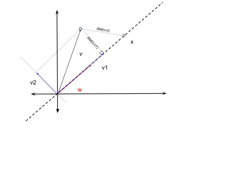
Consider a vector $v \in R^2$. Let $w$ be an arbitrary unit vector in $R^2$, $\Vert w\Vert = 1$. Then the line passing through the origin in the direction of $w$, a 1-D subspace, is given as $L={x \in R^2: x=\alpha w, \alpha \in R}$.

Then, $v=v_1+v_2$, such that $v_1 \in L$ and $v_2 \in L^\perp$.

And the point $v_1$ is closest to $v$ in $L$, $dist(v,x) \geq dist(v,v_1), \forall x \in L$.

The vector $v_1$ is given as $v_1=ww^Tv$. The magnitude of the projected vector is given by $\langle v,w \rangle$.

In general, the orthogonal projection of a vector $v \in R^n$ in m-dimensional subspace $W$ is given as,

where $\beta = \lbrace w_1, w_2…w_m \rbrace $, is the orthonormal basis of $W$. It can be derived directly from the proof of Theorem 1.

Derivation of PCA

Before we consider reduction from higher n-dimension space to lower q-dimension space, we look at a one-dimensional projection. That is, we have n-dimensional feature vectors, and we want to project them onto a line through the origin. We are trying to find a best-fit line representing all sample data points.

Let the line be in the direction of a unit vector $w$.

The error of the fit is given by the Euclidean distance between the projection and the original data point. That is, if $x$ is a data point in $R^n$, then the error of projecting is given as $\Vert x - ww^Tx\Vert $.

Consider our data as $m$ samples of $n$-dimensional feature space ($R^n$). Let $x_i$ denote the $i^{th}$ sample.

Then the mean square error of the projection is given as,

After simplification,

Our objective is to find such $w$ that minimizes the $MSE$. This is equivalent to maximising $\frac{1}{m}\sum_{i=1}^{m}{\langle x_i,w \rangle^2}$.

We can see that $\frac{1}{m}\sum_{i=1}^{m}{\langle x_i,w \rangle^2}$ is the square of sample mean of random variable $z_i = \langle x_i,w \rangle$.

$z_i$ is the representation of $x_i$ in the 1-D space.

If we have a centered data, that is, the mean, $\frac{1}{m}\sum_{i=1}^{m}x_i = 0$

Then,

Note: The data being centered is a very important assumption. If not, the data should be centered by subtracting the samples with mean, that is, $x_i:=x_i-\mu$.

We now move ahead with the assumption, that our data is centered.

Therefore, in order to minimize the $MSE$, we have to maximize the sample variance of $z$. Which is the variance along the line onto which our data is projected. This is a strong assertion, we have to see if it generalizes to projecting the data to more than one principal component.

In general, we are trying to project the n-dimensional data into a lower dimensional subspace of dimension $q$, such that $MSE$ is minimum. We have shown before that for any data point, the closest representation of the data point in subspace of lower dimension is its orthogonal projection onto it. The question is which is the right subspace.

Let the orthonormal basis of the subspace of dimension $p$, $p < n$, be $\beta = {w_1, w_2…w_p}$. The basis vectors are known as the principal components. The projected data can be represented by the p-dimensional coordinates given by $z_i = [z_{i1}, z_{i2},…z_{ip}]^T$, where $z_{ij} = \langle x_i, w_j \rangle$, which is the projection along direction $w_j$.

In order to find the right subspace, we have to solve the following optimization problem associated with it:

Minimize: $\frac{1}{m} \sum_{i=1}^{m} {\Vert x_i - \sum_{j}^{p}{w_j w_j^T x_i}\Vert }^2$

Constraint: $\beta = \lbrace w_1, w_2…w_p \rbrace$ is an orthonormal basis.

If we expand the expression, a lot of cross product terms will cancel out. Recall the fact that the square of norm of sum of orthogonal vectors, is the sum of squares of norms of the two vectors. (Result 3)

Therefore,

Therefore, the $MSE$ is given by,

We can see that, minimizing $MSE$ is same as maximizing $\frac{1}{m} \sum_{i=1}^{m}\Vert \sum_{j}^{p}{w_j w_j^T x_i}\Vert ^2$

By applying (Result 3),

Therefore, we have to maximize the expression $\frac{1}{m} \sum_{j}^{p}{\sum_{i=1}^{m}\langle x_i,w_j \rangle}^2$.

This expression is similar to the case of projecting to a line. Therefore by trying to maximize the sum for each component $j$, we are left with maximizing the sum of the sample variances of the projections on each of the components.

Maximize:

The only constraint is the fact that all $w_j$’s form an orthonormal basis.

If we could maximize the sum of variances without violating the constraint then we essentially have a solution for our optimization problem.

Before going any further we will look at some statistical concepts which are required.

Key statistical concepts

Definition: The expected value of a random matrix $\mathbf{X}$ is given as a matrix such that the entries of $E(\mathbf{X})$ are the expected values respective entries of $\mathbf{X}$

The linearity of the expectation operator easily follows from this definition, which is stated below.

Theorem 2: Let $W_1$ and $W_2$ be m x n matrices of random variables, let $A_1$ and $A_2$ be k x m matrices of constants, and let $B$ be an n x l matrix of constants. Then

Definition: Let $X = [X_1,X_2..X_n]^T$ be n x 1 vector. It’s covariance matrix is defined as

We can see that $Cov(X)_{ij} = Cov(X_i, X_j)$ (Covariance matrix is a symmetric matrix)

Upon further algebraic manipulation, along with linearity of expectation, we get alternative expression for $Cov(X)$ as

Theorem 3: Let $A$ be an m x n matrix of constants. Then

The proof is straightforward. We can get this result by using the alternative expression of covariance and the linearity of expectation.

Theorem 4: $Cov(X)$ is a positive semi-definite matrix.

Proof: Consider an arbitrary vector $Z \in R^n$. Then we know that the variance of $Z^TX$ is non-negative. Therefore,

We already know that $Cov(X)$ is symmetric. Therefore, $Cov(X)$ is positive semi-definite.

Note: For sample covariance matrix, we replace the covariances with sample covariances of respective entries. We can similarly show that sample covariance matrix is a positive semi-definite matrix.

Maximizing the sum of variances

Let $\mathbf{X}$ denote the entire data. The rows of $\mathbf{X}$ are the n-dimensional data points, which are denoted as $x_i$.

Since we have assumed the data to be centered, sample covariance matrix is given as

Consider the expression $\sum_{i}^{m}\langle x_i,w_j \rangle^2$

The sample variance along each principal component $j$ is given below.

Returning back to the optimization problem

The Lagrange function is given as

with $w_j^T w_j = 1$ for all j.

By taking the gradient with respect to $w_j$ and equating to zero we get

Thus, desired vector $w_j$ is an eigenvector of the covariance matrix C.

Also, $L = \sum_{j=1}^{p} \lambda_j$.

Since C is a symmetric matrix, it has a singular value decomposition same as the eigenvalue decomposition.

That is,

$\Sigma$ is the diagonal matrix consisting of all the eigenvalues of C arranged in decreasing order from top to bottom. The columns of $\Lambda$ forms an orthonormal basis of $R^n$.

Thus, if we select the first $p$ eigenvalues, and the first $p$ columns of $\Lambda$, we get the $p$ principal components and the variances of projections along them (eigenvalues).

Encoder Decoder Architecture

For any $x \in R^n$, after subtracting the mean, $x := x - \mu$, It could be easily transformed (encoded) in a lower dimenison representation $z \in R^k$ given by the first k principal components $[w_1, w_2 .. w_k]$.

Similarly, it could be decoded again,

Python Implementaion

I have created a notebook containing the PCA implementation. It is done using only the NumPy library of python. Check out my demo notebook here.

Caveats

PCA, a method for reducing dimensionality, often faces limitations due to its reliance on linear transformations. This involves projecting data from a higher-dimensional space to a lower-dimensional one using a projection matrix composed of principal components. To illustrate, imagine a scenario where data is generated in two dimensions as $x = [x_1, x_1^2]$, causing all points to lie on a parabolic curve. In this context, achieving a reduction without loss demands a non-linear approach. This can be achieved by employing an encoding function $f(x) = x_1$ and a decoding function $g(x) = [x, x^2]$. The potential for greater flexibility arises with intricate non-linear transformations, possibly in the form of a sequence of such transformations through neural networks.

Autoencoders expand upon this concept by utilizing neural networks to tackle the limitations of linear transformations observed in methods like PCA. Unlike PCA, autoencoders can capture intricate non-linear relationships within data. An autoencoder consists of an encoder and a decoder. The encoder function, typically a neural network, maps the input data into a lower-dimensional representation, effectively compressing it. The decoder function, another neural network, then reconstructs the original data from this compressed representation.

Another point to consider is that gaining an understanding of representations is often complex; just aiming to learn a condensed form with maximum variability doesn’t guarantee optimal distinctiveness.

In conclusion, even though PCA might appear antiquated, it still serves as a valuable initial step in the journey of understanding representation learning.

Further reading

• Notes written by Yang Xu for 10-701 Machine Learning (Spring 2012) Principal Component Analysis.

• A good summary paper on Autoencoders