Variational Autoencoders

Variational Autoencoders (VAEs) represent a fundamental breakthrough in generative modeling, combining the power of deep neural networks with principled Bayesian inference. Introduced by Kingma and Welling (2013) [1], VAEs provide a scalable framework for learning complex probabilistic models with continuous latent variables.

The Latent Variable Model

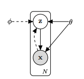
The following generative process is assumed, first sample $z \sim p_\theta(z)$. Then sample x from $p_\theta(x\vert z)$.

The Bayes’ rule gives the joint distribution for the generative model.

Likelihood optimization

In order to optimize the parameters of our generative model, we assume that the training set consists of i.i.d. observations coming from $p_{data}$. We would then maximise the (log) likelihood of our model. If the marginal $p_\theta(x)$ were tractable, then we would be done. Unfortunately, this is most of the time not possible.

Let’s concentrate on the expression $log p_\theta (x)$ (i.e., the likelihood of a single example). It simplifies into the following:

Estimating the gradient of the expression w.r.t $\theta$ using a Monte Carlo estimation is not straightforward. (But it could be done, using a re-parameterization trick or log-derivative trick etc.) For simplicity, we often assume prior being parameter-free (i.e., $z \sim p(z)$). We can now resort to just taking the average of $p_\theta(x\vert z)$ sampled from $z \sim p(z)$. However, this is been found to be practically inefficient due to large variance. To reduce the variance and make the estimation more precise, we utilize importance sampling:

In this approach, the average is taken of the quantity inside expectation over samples drawn from $q(z)$. The variance of the estimate depends on the choice of $q(z)$ and is given by:

For zero variance, we would like $q(z) \propto p_\theta(x\vert z) p_\theta(z) $. We can then show that it is equivalent to saying $q(z) = p_{\theta}(z \vert x)$:

In practice, the closer $q(z)$ is to the posterior ($p_{\theta}(z \vert x))$, the faster the convergence and better the estimate.

Our discussion so far has provided two optimization objectives to improve our generative model given a single datapoint $x$:

Objective (1): Maximize Likelihood

A lower bound for this expression could be obtained using Jensen’s Inequality:

It is easy to verify that the equality holds when $q(z) \propto p_\theta(x \vert z) p_\theta(z)$. This aligns well with our second objective.

Objective (2): We would like to make $q(z)$ close to the posterior.

We would like to maximize Objective 1 and minimize Objective 2, we may roughly obtain a good solution if we try to maximise (Obj 1 - Obj 2). Let’s consider the term which we would get if we subtract the two objectives (Obj 1 - Obj 2):

We can observe that this term is exactly the same as the lower bound for likelihood obtained by the implementation of Jensen’s inequality. This alignment is not accidental. In fact, our entire previous discussion merged two distinct viewpoints into a single one, ultimately leading us to the ELBO function.

Amortised Inference

When maximizing the ELBO w.r.t $\theta$ and $q$, The inference distribution $q(z)$ has to be optimized, for each $x$ individually, and it’s computationally expensive. Ideally, we aim to learn a mapping instead, allowing us to pass an unseen $x$ as input and obtain the corresponding distribution without the need for costly individual optimization. The distribution is parameterized by $\phi$ (i.e., $z \sim q_\phi(z \vert x)$).

The log-likelihood for the entire training batch $D$ is sum of individual likelihood, hence the sum of ELBO loss over all the points serve as the lower bound.

The objective function to optimize would be: \(L(\theta,\phi,D) = \sum_{x_i \in D} \ell(\theta,\phi,x_i)\)

Where \(\ell(\theta,\phi,x) = E_{z \sim q_\phi(z \vert x)} \left[\log \frac {p_\theta(x,z) }{q_\phi(z \vert x)} \right]\)

$\beta$-VAE

After performing some algebraic manipulations, it’s easy to see,

Since we are trying to maximize the objective, The terms within the bracket need to be minimized. The first part of the expression is also called the reconstruction error (cross-entropy). The second part is known as a regularizing term. By trying to optimize our objective, we are in essence trying to minimize the reconstruction error of our encoding decoding scheme and making sure that the inference distribution $q$ stays close to prior $p$.

Both terms are important for the objective. To see why, imagine you’re generating a new data point $x$ with a trained VAE. First, you sample $z$ from $p(z)$, and then you generate $x$ based on $p(x \vert z)$. What’s crucial to recognize is that we’re effectively sampling $(x, z)$ from $p_\theta(x, z)$, rather than directly generating $x$ from $p_\theta(x)$. This makes sense because if you think of a manifold in $x$ space that houses all the true data points, $q(z \vert x)$ establishes a kind of mapping. The regularization term in our objective ensures that $q(z \vert x)$ stays close to $p(z)$, letting us select a $z$ that can be decoded to a meaningful $x$. Reconstruction loss is important as well. Otherwise, our encoder-decoder scheme would simply fail.

In Beta-VAE [2], the loss function is modified as follows:

It provides a control to balance between the quality of data reconstruction and the structure of the latent representation. A low $\beta$ focuses on better reconstruction, whereas a high $ \beta$ emphasizes a better-structured latent space (closeness to the choice of prior).

The choice of $\beta$ has profound implications for representation learning. Since the prior is typically a standard Gaussian, increasing $\beta$ forces the encoder distribution $q_\phi(z \vert x)$ to more closely approximate this standard Gaussian. When we prioritise the KL-divergence term with a high $\beta$ value, the encoder learns to produce more disentangled representations. This means $q_\phi(z \vert x)$ approaches a standard Gaussian where each latent dimension becomes approximately independent of the others, leading to disentangled factors of variation in the learned representation. However, this comes with a trade-off: higher $\beta$ values can lead to poor reconstruction.

The Challenge of Gradient Estimation with Expectations

In many situations while performing gradient descent, we often come across taking a gradient over a loss which constitutes an expectation term. Since most of the time the integral calculation is not tractable, we resort to sampling as an approximation.

Recalling Leibniz rule from multivariate calculus, if $F(\theta)$ is defined by the integral:

Then the derivative of $F$ with respect to $\theta$ is given by:

For our purpose, let $F$ be $\mathbb{E}{x \sim p\theta}[f(x,\phi)]$:

Then calculating $\nabla_\phi F$ (gradient w.r.t $\phi$) is straightforward:

This can be approximated by sampling. The more challenging situation is calculating $\nabla_\theta F$:

Notice that this time the gradient is not inside an expectation with respect to the distribution $p_\theta$, so the integral cannot be approximated by sampling from $p$.

There are many tricks in the literature to overcome this challenge [3], and reparameterization is one of the key techniques applied in VAE loss calculations. The emphasis of various tricks is upon the convergence of estimates and ease of calculation.

One simple trick is to replace the gradient of density with the log of density times the density:

Hence the gradient $\nabla_\theta F$ can be rewritten as:

This is known as the REINFORCE estimator or score function estimator, but it often has high variance in practice.

The Reparameterization Trick

The reparameterization trick provides an elegant solution to the gradient estimation problem by transforming the sampling process. Instead of sampling directly from $p_\theta(x)$, we express $x$ as a deterministic function of $\theta$ and a noise variable $\epsilon$.

The Core Idea

The key insight is to reparameterize $x$ as:

where $\epsilon \sim p(\epsilon)$ is sampled from a simple distribution (like standard normal), and $g_\theta$ is a deterministic function parameterized by $\theta$.

If we can write $x = g_\theta(\epsilon)$ where $\epsilon \sim p(\epsilon)$, then:

Now we can compute the gradient:

This gradient can now be estimated by sampling $\epsilon$ from the simple distribution $p(\epsilon)$.

Example: Gaussian Distribution

For a Gaussian distribution $\mathcal{N}(\mu, \sigma^2)$, we can reparameterize as:

where $\epsilon \sim \mathcal{N}(0,1)$. This allows us to:

1. Sample $\epsilon$ from standard normal
2. Transform it deterministically to get $x$
3. Compute gradients with respect to $\mu$ and $\sigma$ through the deterministic transformation

Application in VAEs

In VAEs, we have an encoder that produces parameters of a distribution $q_\phi(z \vert x)$, and we need to compute:

Using the reparameterization trick:

1. The encoder outputs $\mu(x)$ and $\sigma(x)$
2. We sample $\epsilon \sim \mathcal{N}(0,I)$
3. We compute $z = \mu(x) + \sigma(x) \odot \epsilon$
4. We can now backpropagate through this deterministic computation

The reparameterization trick requires that we can express the distribution as a deterministic transformation of a simple noise source. This works well for:

• Gaussian distributions
• Uniform distributions
• Some exponential family distributions

But may not be directly applicable to discrete distributions or more complex continuous distributions.

References

[1] Kingma, D. P., & Welling, M. (2013). Auto-Encoding Variational Bayes. arXiv preprint arXiv:1312.6114.

[2] Burgess, C.P., Higgins, I., Pal, A., Matthey, L., Watters, N., Desjardins, G. and Lerchner, A., 2018. Understanding disentangling in $\beta $-VAE. arXiv preprint arXiv:1804.03599.

[3] Walder, C.J., Roussel, P., Nock, R., Ong, C.S. and Sugiyama, M., 2019. New tricks for estimating gradients of expectations. arXiv preprint arXiv:1901.11311.